Multipanel figures with ggplot2
Multipanel figures — where several plots are arranged together into a single figure — are a common way to present related results side by side. In R with ggplot2, there are two main approaches:
- Faceting, which splits a single dataset into panels based on the values of one or more variables.
- Combining separate plots using the patchwork package, which lets you arrange completely independent ggplots together.
Before you get started, read the page on the basics of plotting with ggplot and install the package ggplot2.
library(ggplot2)For the examples on this page we will use the iris dataset (already built into R) and the mpg dataset from ggplot2.
data(iris)
data(mpg)
Faceting with facet_wrap
Faceting is ideal when you want to make the same type of plot for subsets of your data. facet_wrap takes a single grouping variable and wraps the panels into rows and columns automatically.
The formula syntax ~ variable specifies which variable to split on. For example, to make a separate scatter plot for each iris species:
p <- ggplot(iris, aes(Sepal.Length, Petal.Length)) +
  geom_point() +
  theme_classic()

p + facet_wrap(~ Species)
By default facet_wrap tries to make the panel layout as square as possible. You can control the number of rows or columns with nrow or ncol:
p + facet_wrap(~ Species, ncol = 1)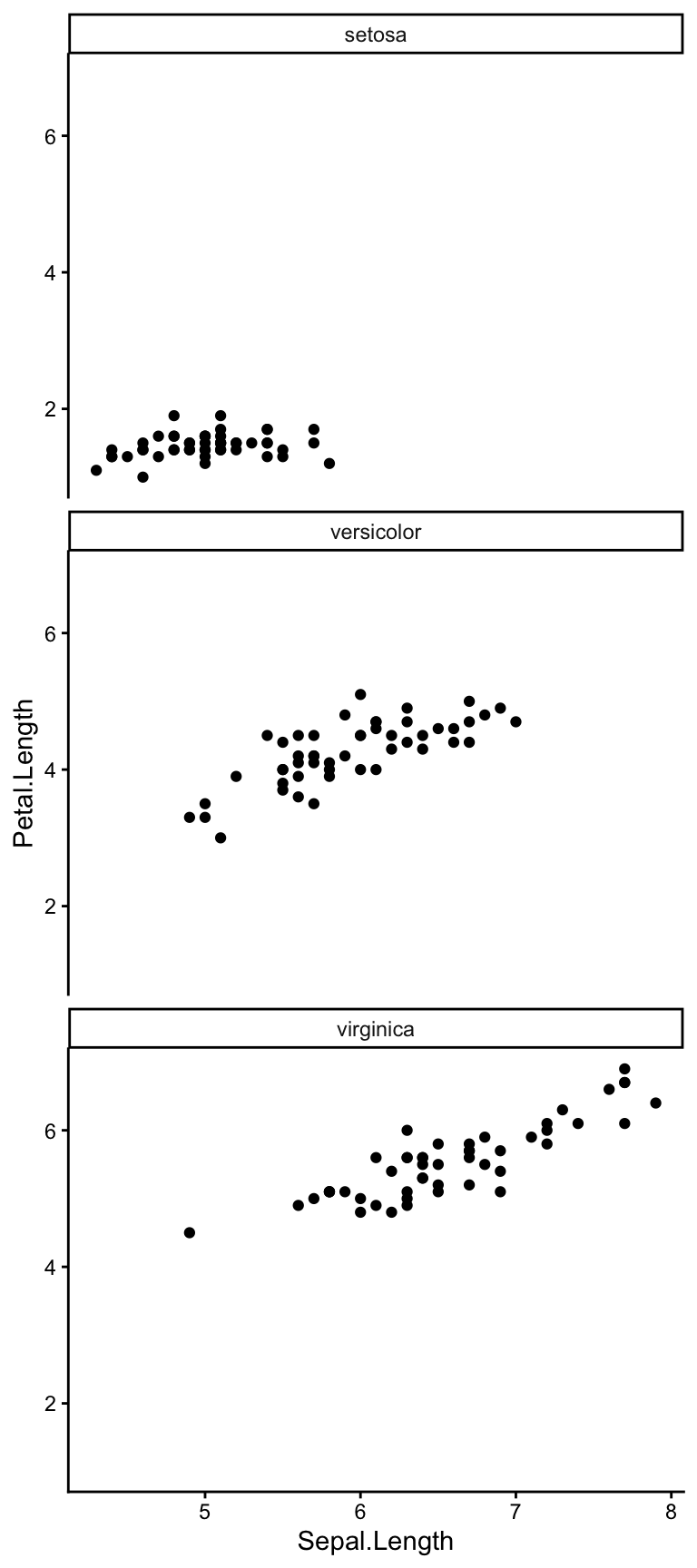
You can add scales = "free" if you want each panel to use its own axis limits, rather than sharing the same scale across all panels. This is useful when the ranges differ greatly between groups, but makes direct visual comparison harder.
p + facet_wrap(~ Species, scales = "free")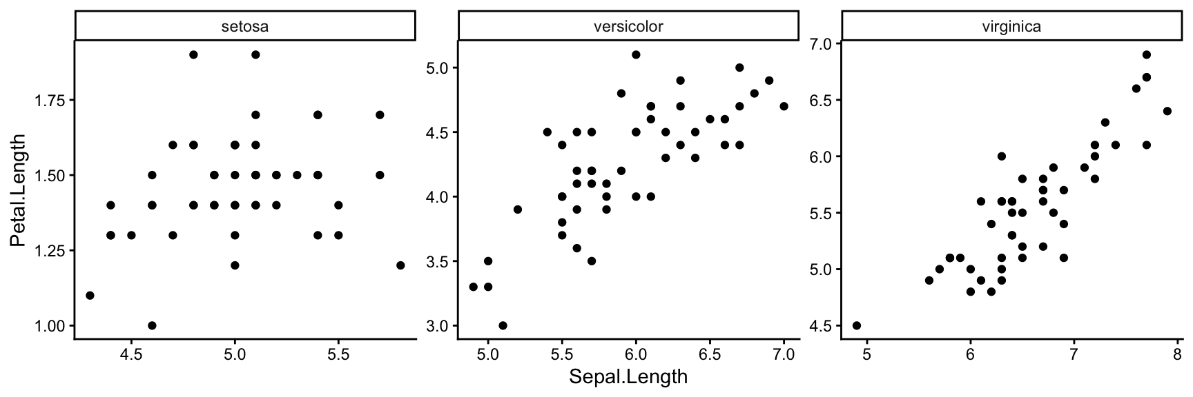
Faceting with facet_grid
facet_grid lays panels out in a strict grid defined by two variables — one for rows and one for columns. Use the formula rows ~ cols. To facet only on one dimension, replace the other with a dot (.).
Here we use the mpg dataset, splitting by drive type (drv) in rows and number of cylinders (cyl) in columns:
ggplot(mpg, aes(displ, hwy)) +
  geom_point() +
  theme_classic() +
  facet_grid(drv ~ cyl)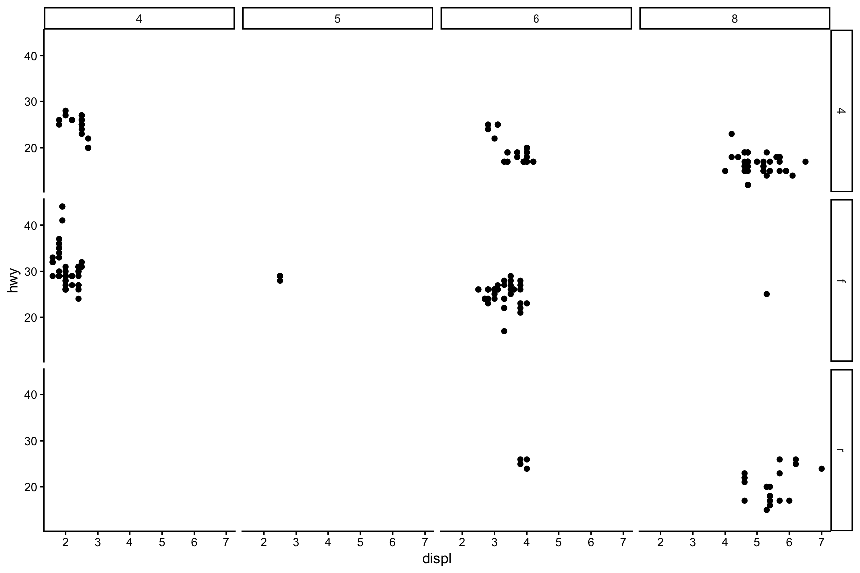
facet_grid is useful when you have two categorical variables and want to see every combination. Empty panels appear where no data exist for a given combination.
To facet on just one variable across rows with facet_grid, use . ~ variable (or variable ~ . for columns):
ggplot(mpg, aes(displ, hwy)) +
  geom_point() +
  theme_classic() +
  facet_grid(. ~ drv)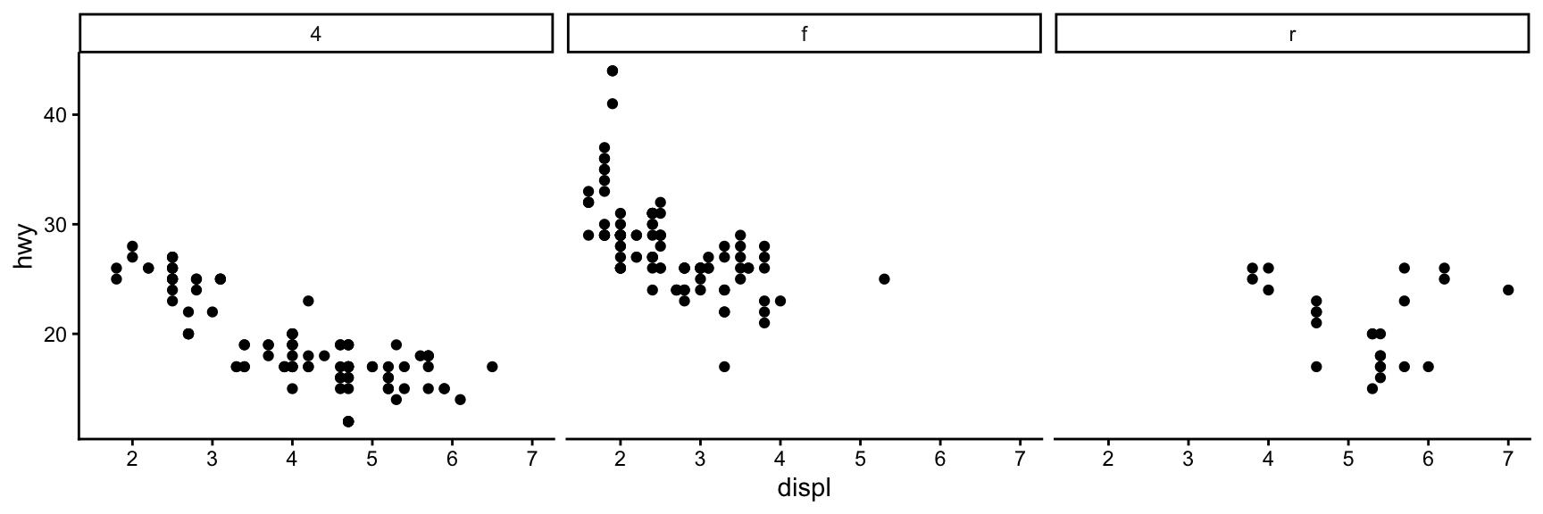
Customising facet labels and strips
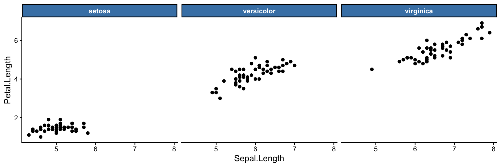
By default the facet labels are the values of the grouping variable. You can change the strip background and text colour inside a theme() call:
p + facet_wrap(~ Species) +
  theme(
    strip.background = element_rect(fill = "steelblue"),
    strip.text = element_text(colour = "white", face = "bold")
  )
To rename the labels without changing the underlying data, supply a named character vector to the labeller argument:
species_labels <- c(
  setosa = "I. setosa",
  versicolor = "I. versicolor",
  virginica = "I. virginica"
)

p + facet_wrap(~ Species, labeller = labeller(Species = species_labels)) +
  theme(strip.text = element_text(face = "italic"))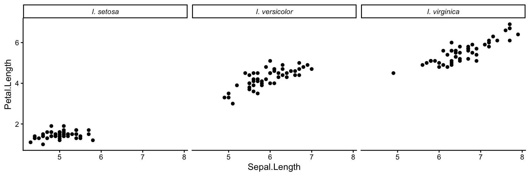
Combining separate plots with patchwork
Faceting requires all panels to share the same underlying ggplot call and the same geom type. When you want to combine different plots — perhaps a scatter plot next to a bar plot — use the patchwork package.
Install it once with install.packages("patchwork"), then load it:
library(patchwork)First, create two separate ggplot objects:
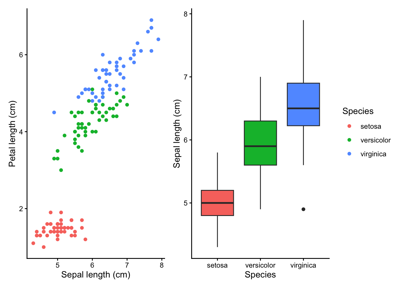
p1 <- ggplot(iris, aes(Sepal.Length, Petal.Length, colour = Species)) +
  geom_point() +
  theme_classic()

p2 <- ggplot(iris, aes(Species, Sepal.Length, fill = Species)) +
  geom_boxplot(show.legend = FALSE) +
  theme_classic()
The | operator places plots side by side, and / stacks them vertically:
p1 | p2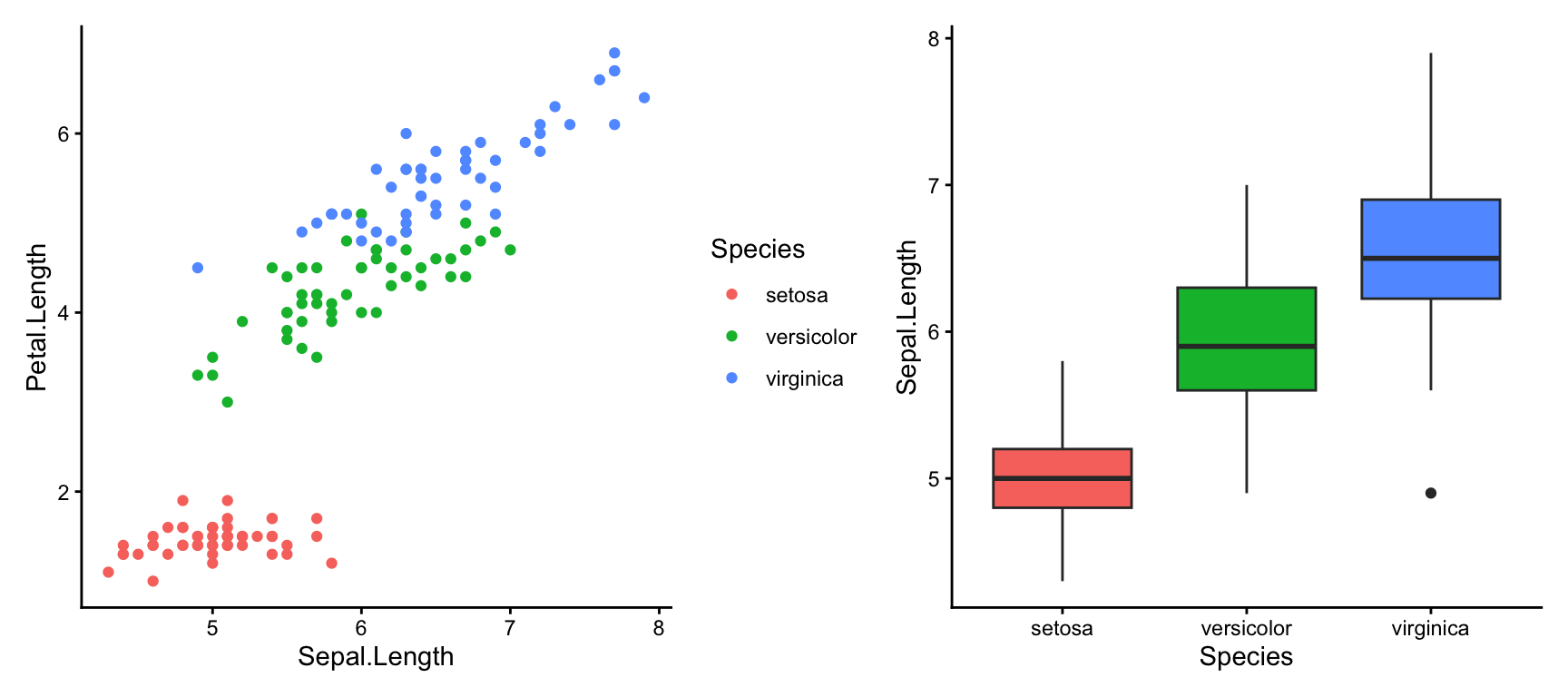
p1 / p2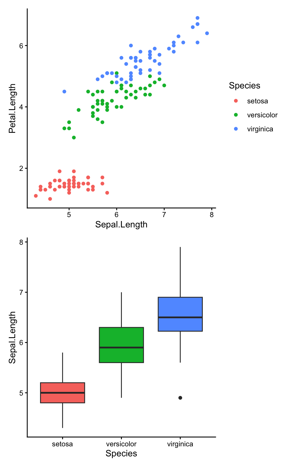
You can mix | and / and use brackets to control grouping. For example, to put two narrow plots on the right and one tall plot on the left:
p3 <- ggplot(iris, aes(Petal.Width, Petal.Length, colour = Species)) +
  geom_point() +
  theme_classic()

p1 | (p2 / p3)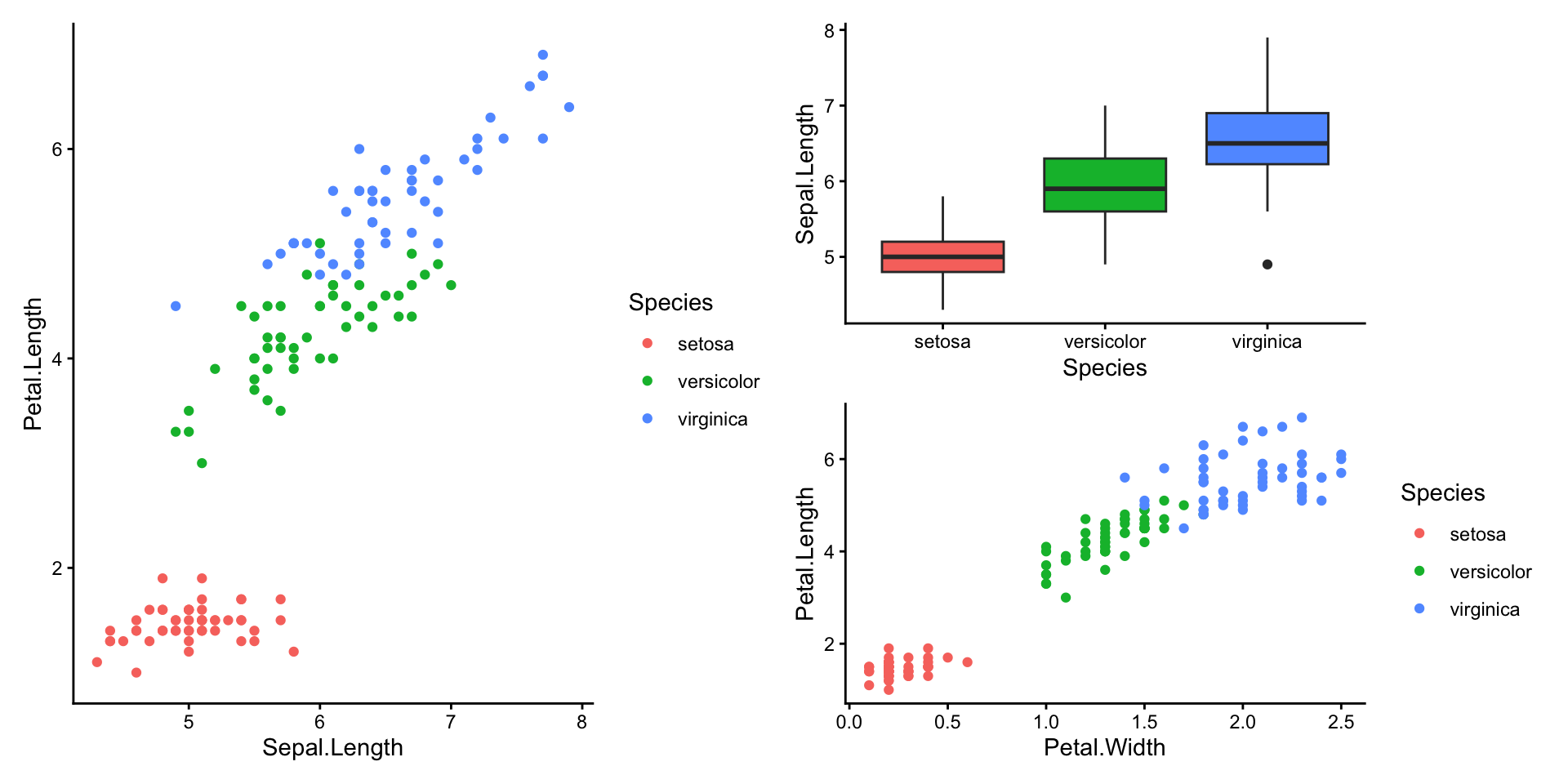
Adding panel labels with patchwork
Publication figures often label each panel with a letter (A, B, C…). patchwork makes this straightforward with plot_annotation:
(p1 | (p2 / p3)) +
  plot_annotation(tag_levels = "A")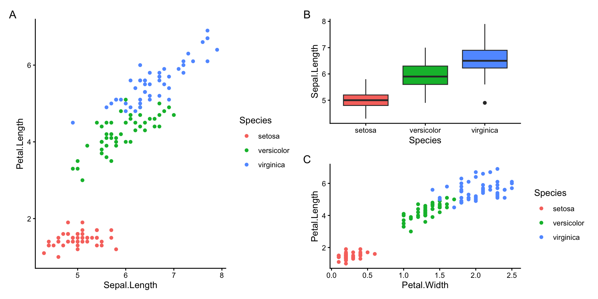
You can also add a shared title across all panels:
(p1 | p2) +
  plot_annotation(
    title = "Iris sepal and petal measurements",
    theme = theme(plot.title = element_text(size = 14, face = "bold"))
  )
## Warning: annotation$theme is not a valid theme.
## Please use `theme()` to construct themes.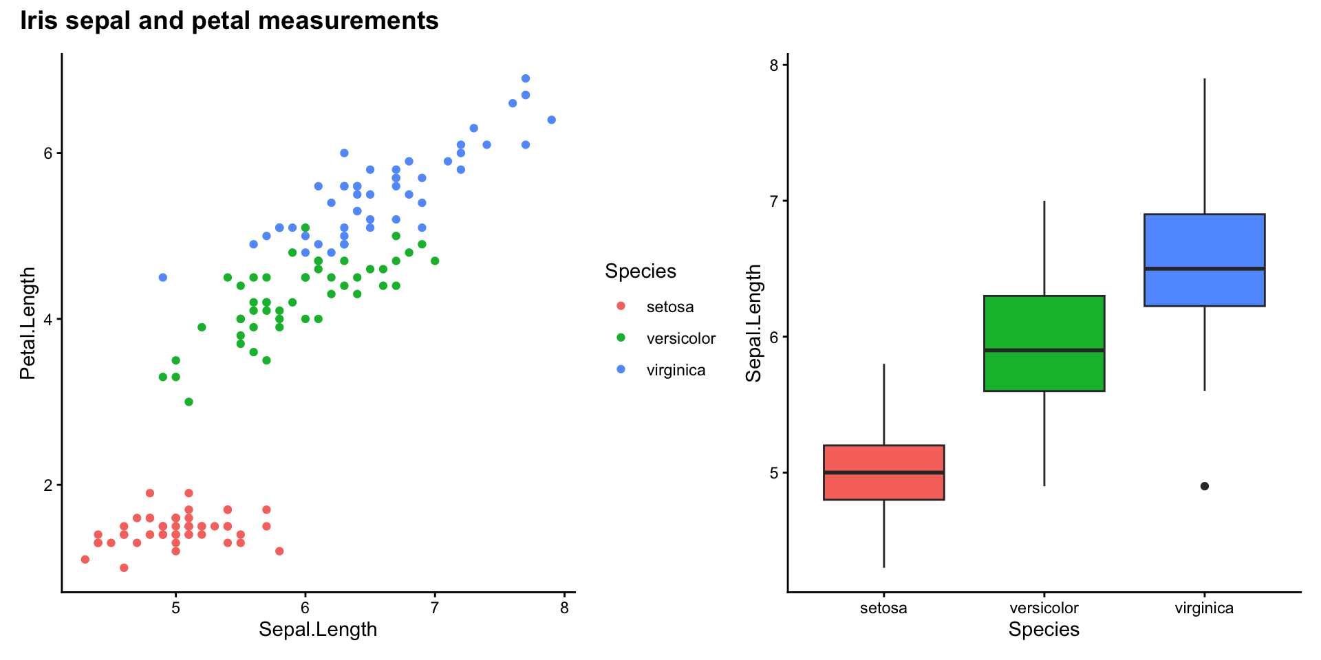
Collecting shared legends
When panels share the same colour or fill aesthetic, patchwork can merge their legends into one with plot_layout(guides = "collect"):
(p1 | p3) +
  plot_layout(guides = "collect")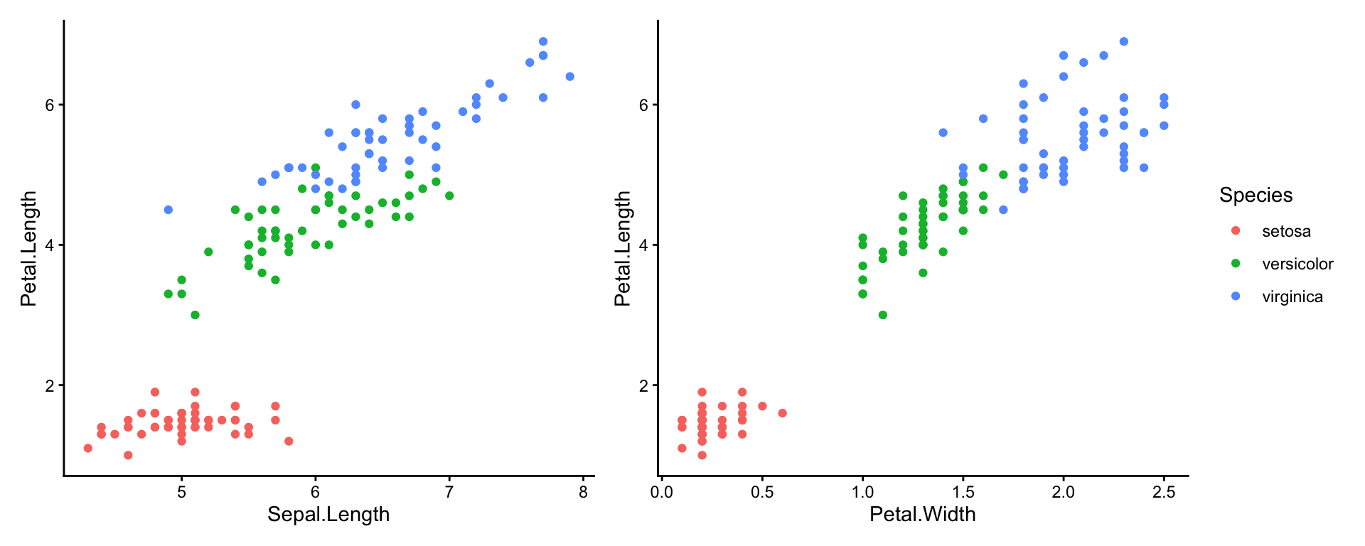
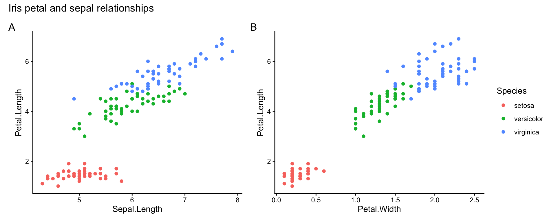
Combine with plot_annotation to get a clean, publication-ready layout in a few lines of code:
(p1 | p3) +
  plot_layout(guides = "collect") +
  plot_annotation(
    tag_levels = "A",
    title = "Iris petal and sepal relationships"
  )
Further help
- Facets chapter in the ggplot2 book
- patchwork documentation — including more advanced layouts with
plot_layout()andinset_element() - Our other ggplot pages:
Pedersen, T L (2024) patchwork: The Composer of Plots. R package. https://patchwork.data-imaginist.com
Wickham, H (2016) ggplot2: Elegant Graphics for Data Analysis. Springer-Verlag New York.
Author: Environmental Computing
Year: 2025
Last updated: Mar 2026